代码演示

PyCharm + Anaconda | 完整代码在最后面

import numpy as np
import matplotlib as mpl
import matplotlib.pyplot as plt

np.random.seed(42)
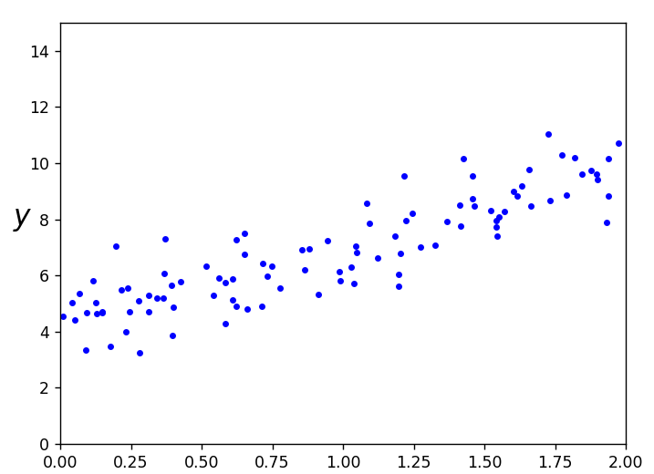
# 生成一个Y = 4 + 3 * X + 高斯噪声的线性数据集
m = 100
X = 2 * np.random.rand(m, 1)
y = 4 + 3 * X + np.random.randn(m, 1)

plt.plot(X, y, "b.")
plt.xlabel("$x_1$", fontsize=18)
plt.ylabel("$y$", rotation=0, fontsize=18)
plt.axis([0, 2, 0, 15])

先看一下显示结果

接下来是训练过程

# 初始参数
n_epochs = 50
t0, t1 = 5, 50


# 学习率函数
def learning_schedule(t):
    return t0 / (t + t1)


# 初始权重，包含偏移量
theta = np.random.randn(2, 1)
# 输入扩展，扩展与偏移量对应的全1列
X_b = np.c_[np.ones((m, 1)), X]

# 训练多个轮次
for epoch in range(n_epochs):
    for i in range(0, m):
        # 随机取一个样本
        random_index = np.random.randint(m)
        xi = X_b[random_index:random_index + 1]
        yi = y[random_index:random_index + 1]
        # 计算梯度
        gradients = 2 * xi.T.dot(xi.dot(theta) - yi)
        eta = learning_schedule(epoch * m + i)
        # 更新权重
        theta = theta - eta * gradients

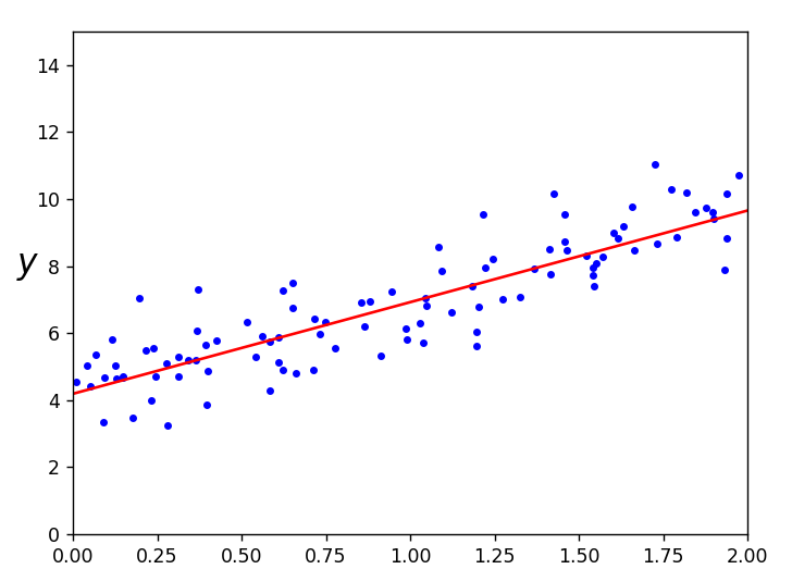
简单的说就是将数据随机选取，分成50轮次训练，每一次都会根据计算的梯度来调整截距和斜率，最后拟合出最佳直线

请看结果：

附录：

import numpy as np
import matplotlib as mpl
import matplotlib.pyplot as plt
np.random.seed(42)

# 生成一个Y = 4 + 3 * X + 高斯噪声的线性数据集
m = 100
X = 2 * np.random.rand(m, 1)
y = 4 + 3 * X + np.random.randn(m, 1)

plt.plot(X, y, "b.")
plt.xlabel("$x_1$", fontsize=18)
plt.ylabel("$y$", rotation=0, fontsize=18)
plt.axis([0, 2, 0, 15])

############################## 手写随机梯度下降法 ##############################
# 初始参数
n_epochs = 50
t0, t1 = 5, 50


# 学习率函数
def learning_schedule(t):
    return t0 / (t + t1)


# 初始权重，包含偏移量
theta = np.random.randn(2, 1)
# 输入扩展，扩展与偏移量对应的全1列
X_b = np.c_[np.ones((m, 1)), X]

# 训练多个轮次
for epoch in range(n_epochs):
    for i in range(0, m):
        # 随机取一个样本
        random_index = np.random.randint(m)
        xi = X_b[random_index:random_index + 1]
        yi = y[random_index:random_index + 1]
        # 计算梯度
        gradients = 2 * xi.T.dot(xi.dot(theta) - yi)
        eta = learning_schedule(epoch * m + i)
        # 更新权重
        theta = theta - eta * gradients

# 预测画出直线
X_Test = [[0], [2]]
Y_Test = X_Test * theta[1] + theta[0]
plt.plot(X_Test, Y_Test, "r-")
print(theta)
print(Y_Test)
plt.show()